Review: If  is normal with mean
  and standard deviation
  , then

is the Standard Normal Distribution with mean 0 and standard deviation 1. To find the probability  , you would convert to the standard normal distribution and look up the values in the standard normal table.

If  is a weighted sum of
  normal random variables
  , with means
  , variance
  , and weights
  , then
![\displaystyle E\left[\sum_{i=1}^n w_iX_i\right] = \sum_{i=1}^n w_i\mu_i](https://s0.wp.com/latex.php?latex=%5Cdisplaystyle+E%5Cleft%5B%5Csum_%7Bi%3D1%7D%5En+w_iX_i%5Cright%5D+%3D+%5Csum_%7Bi%3D1%7D%5En+w_i%5Cmu_i&bg=ffffff&fg=333333&s=0&c=20201002)
and variance

where  is the covariance between
  and
and  . Note when
  ,
,  .
.
Remember: A sum of random variables is not the same as a mixture distribution! The expected value is the same, but the variance is not. A sum of normal random variables is also normal. So is normal with the above mean and variance.
Actuary Speak: This is called a stable distribution. The sum of random variables from the same distribution family produces a random variable that is also from the same distribution family.
The fun stuff:
If is normal, then  is lognormal. If has mean and standard deviation , then
![\begin{array}{rll} \displaystyle E\left[Y\right] &=& E\left[e^X\right] \\ \\ \displaystyle &=& e^{\mu + \frac{1}{2}\sigma^2} \\ \\ Var\left(e^X\right) &=& e^{2\mu + \sigma^2}\left(e^{\sigma^2} - 1\right)\end{array}](https://s0.wp.com/latex.php?latex=%5Cbegin%7Barray%7D%7Brll%7D+%5Cdisplaystyle+E%5Cleft%5BY%5Cright%5D+%26%3D%26+E%5Cleft%5Be%5EX%5Cright%5D+%5C%5C+%5C%5C+%5Cdisplaystyle+%26%3D%26+e%5E%7B%5Cmu+%2B+%5Cfrac%7B1%7D%7B2%7D%5Csigma%5E2%7D+%5C%5C+%5C%5C+Var%5Cleft%28e%5EX%5Cright%29+%26%3D%26+e%5E%7B2%5Cmu+%2B+%5Csigma%5E2%7D%5Cleft%28e%5E%7B%5Csigma%5E2%7D+-+1%5Cright%29%5Cend%7Barray%7D&bg=ffffff&fg=333333&s=0&c=20201002)
Recall  where
where  is the future value of an investment growing at a continuously compounded rate of
  for one period. If the rate of growth is a normal distributed random variable, then the future value is lognormal. The Black-Scholes model for option prices assumes stocks appreciate at a continuously compounded rate that is normally distributed.

where  is the stock price at time
  ,
,  is the current price, and
  is the random variable for the rate of return from time 0 to t. Now consider the situation where is the sum of iid normal random variables
  each having mean
  and variance
  . Then
![\begin{array}{rll} E\left[R(0,t)\right] &=& n\mu_h \\ Var\left(R(0,t)\right) &=& n\sigma_h^2 \end{array}](https://s0.wp.com/latex.php?latex=%5Cbegin%7Barray%7D%7Brll%7D+E%5Cleft%5BR%280%2Ct%29%5Cright%5D+%26%3D%26+n%5Cmu_h+%5C%5C+Var%5Cleft%28R%280%2Ct%29%5Cright%29+%26%3D%26+n%5Csigma_h%5E2+%5Cend%7Barray%7D&bg=ffffff&fg=333333&s=0&c=20201002)
If  represents 1 year, this says that the expected return in 10 years is 10 times the one year return and the standard deviation is
  times the annual standard deviation. This allows us to formulate a function for the mean and standard deviation with respect to time. Suppose we write
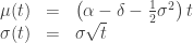
where  is the growth factor and is the continuous rate of dividend payout. Since all normal random variables are transformations of the standard normal, we can write
 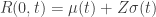 . The model for the stock price becomes

In this model, the expected value of the stock price at time is
![E\left[S_t\right] = S_0e^{(\alpha - \delta)t}](https://s0.wp.com/latex.php?latex=E%5Cleft%5BS_t%5Cright%5D+%3D+S_0e%5E%7B%28%5Calpha+-+%5Cdelta%29t%7D&bg=ffffff&fg=333333&s=0&c=20201002)
Actuary Speak: The standard deviation of the return rate is called the volatility of the stock. This term comes from expressing the rate of return as an Ito process.  is called the drift term and
  is called the volatility term.
Confidence intervals: To find the range of stock prices that corresponds to a particular confidence interval, we need only look at the confidence interval on the standard normal distribution then translate that interval into stock prices using the equation for .
Example: For example ![z=[-1.96, 1.96]](https://s0.wp.com/latex.php?latex=z%3D%5B-1.96%2C+1.96%5D&bg=ffffff&fg=333333&s=0&c=20201002) represents the 95% confidence interval in the standard normal
represents the 95% confidence interval in the standard normal  . Suppose
  ,
,  ,
,  ,
,  , and
, and  . Then the 95% confidence interval for is
![\left[40e^{(0.15-0.01-\frac{1}{2}0.3^2)\frac{1}{3} + (-1.96)0.3\sqrt{\frac{1}{3}}},40e^{(0.15-0.01-\frac{1}{2}0.3^2)\frac{1}{3} + (1.96)0.3\sqrt{\frac{1}{3}}}\right]](https://s0.wp.com/latex.php?latex=%5Cleft%5B40e%5E%7B%280.15-0.01-%5Cfrac%7B1%7D%7B2%7D0.3%5E2%29%5Cfrac%7B1%7D%7B3%7D+%2B+%28-1.96%290.3%5Csqrt%7B%5Cfrac%7B1%7D%7B3%7D%7D%7D%2C40e%5E%7B%280.15-0.01-%5Cfrac%7B1%7D%7B2%7D0.3%5E2%29%5Cfrac%7B1%7D%7B3%7D+%2B+%281.96%290.3%5Csqrt%7B%5Cfrac%7B1%7D%7B3%7D%7D%7D%5Cright%5D&bg=ffffff&fg=333333&s=0&c=20201002)
Which corresponds to the price interval of
![\left[29.40,57.98\right]](https://s0.wp.com/latex.php?latex=%5Cleft%5B29.40%2C57.98%5Cright%5D&bg=ffffff&fg=333333&s=0&c=20201002)
Probabilities: Probability calculations on stock prices require a bit more mental gymnastics.

Conditional Expected Value: Define
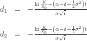
Then
![\begin{array}{rll} \displaystyle E\left[S_t|S_t<K\right] &=& S_0e^{(\alpha - \delta)t}\frac{\mathcal{N}(-d_1)}{\mathcal{N}(-d_2)} \\ \\ \displaystyle E\left[S_t|S_t>K\right] &=& S_0e^{(\alpha - \delta)t}\frac{\mathcal{N}(d_1)}{\mathcal{N}(d_2)} \end{array}](https://s0.wp.com/latex.php?latex=%5Cbegin%7Barray%7D%7Brll%7D+%5Cdisplaystyle+E%5Cleft%5BS_t%7CS_t%3CK%5Cright%5D+%26%3D%26+S_0e%5E%7B%28%5Calpha+-+%5Cdelta%29t%7D%5Cfrac%7B%5Cmathcal%7BN%7D%28-d_1%29%7D%7B%5Cmathcal%7BN%7D%28-d_2%29%7D+%5C%5C+%5C%5C+%5Cdisplaystyle+E%5Cleft%5BS_t%7CS_t%3EK%5Cright%5D+%26%3D%26+S_0e%5E%7B%28%5Calpha+-+%5Cdelta%29t%7D%5Cfrac%7B%5Cmathcal%7BN%7D%28d_1%29%7D%7B%5Cmathcal%7BN%7D%28d_2%29%7D+%5Cend%7Barray%7D&bg=ffffff&fg=333333&s=0&c=20201002)
This gives the expected stock price at time given that it is less than  or greater than respectively.
Black-Scholes formula: A call option  on stock has value
  at time . The option pays out if
  . So the value of this option at time 0 is the probability that it pays out at time , discounted by the risk free interest rate
  , and multiplied by the expected value of
  given that . In other words,
![\begin{array}{rll} \displaystyle C_0 &=& e^{-rt}Pr\left(S_t>K\right)E\left[S_t-K|S_t>K\right] \\ \\ &=& e^{-rt}\mathcal{N}(d_2)\left(E\left[S_t|S_t>K\right] - E\left[K|S_t>K\right]\right) \\ \\ &=& e^{-rt}\mathcal{N}(d_2)\left(S_0e^{(\alpha - \delta)t}\frac{\mathcal{N}(d_1)}{\mathcal{N}(d_2)} - K\right) \end{array}](https://s0.wp.com/latex.php?latex=%5Cbegin%7Barray%7D%7Brll%7D+%5Cdisplaystyle+C_0+%26%3D%26+e%5E%7B-rt%7DPr%5Cleft%28S_t%3EK%5Cright%29E%5Cleft%5BS_t-K%7CS_t%3EK%5Cright%5D+%5C%5C+%5C%5C+%26%3D%26+e%5E%7B-rt%7D%5Cmathcal%7BN%7D%28d_2%29%5Cleft%28E%5Cleft%5BS_t%7CS_t%3EK%5Cright%5D+-+E%5Cleft%5BK%7CS_t%3EK%5Cright%5D%5Cright%29+%5C%5C+%5C%5C+%26%3D%26+e%5E%7B-rt%7D%5Cmathcal%7BN%7D%28d_2%29%5Cleft%28S_0e%5E%7B%28%5Calpha+-+%5Cdelta%29t%7D%5Cfrac%7B%5Cmathcal%7BN%7D%28d_1%29%7D%7B%5Cmathcal%7BN%7D%28d_2%29%7D+-+K%5Cright%29+%5Cend%7Barray%7D&bg=ffffff&fg=333333&s=0&c=20201002)
Black-Scholes makes the additional assumption that all investors are risk neutral. This means assets do not pay a risk premium for being more risky. Long story short,  so
so  . So in the Black-Scholes formula:

Continuing our derivation of  but replacing with ,

For a put option  with payout
  for
for  and 0 otherwise,

These are the famous Black-Scholes formulas for option pricing. When derived on the back of a cocktail napkin, they are indispensable for impressing the ladies at your local bar. :p


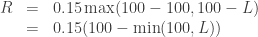
![E[R] = 0.15(100 - E[L \wedge 100])](https://s0.wp.com/latex.php?latex=E%5BR%5D+%3D+0.15%28100+-+E%5BL+%5Cwedge+100%5D%29&bg=ffffff&fg=333333&s=0&c=20201002)
 on an insurance policy that you’ve written, what fraction of expected losses do you eliminate from your expected liability? This is measured by the Loss Elimination Ratio
  .
.![\displaystyle LER(d) = \frac{E\left[X \wedge d\right]}{E\left[X\right]}](https://s0.wp.com/latex.php?latex=%5Cdisplaystyle+LER%28d%29+%3D+%5Cfrac%7BE%5Cleft%5BX+%5Cwedge+d%5Cright%5D%7D%7BE%5Cleft%5BX%5Cright%5D%7D&bg=ffffff&fg=333333&s=0&c=20201002)
 — The payment made by the writer of the policy is the complete amount of the loss
  is the inflation adjusted loss variable. If losses
  are subject to deductible
 ![\begin{array}{rll} \displaystyle LER_Y(d) &=& \frac{E\left[(1+r)X\wedge d\right]}{E\left[(1+r)X\right]} \\ \\ \displaystyle &=&\frac{(1+r)E\left[X\wedge \frac{d}{1+r}\right]}{(1+r)E\left[X\right]} \\ \\ &=& \frac{E\left[X \wedge \frac{d}{1+r}\right]}{E\left[X\right]}\end{array}](https://s0.wp.com/latex.php?latex=%5Cbegin%7Barray%7D%7Brll%7D+%5Cdisplaystyle+LER_Y%28d%29+%26%3D%26+%5Cfrac%7BE%5Cleft%5B%281%2Br%29X%5Cwedge+d%5Cright%5D%7D%7BE%5Cleft%5B%281%2Br%29X%5Cright%5D%7D+%5C%5C+%5C%5C+%5Cdisplaystyle+%26%3D%26%5Cfrac%7B%281%2Br%29E%5Cleft%5BX%5Cwedge+%5Cfrac%7Bd%7D%7B1%2Br%7D%5Cright%5D%7D%7B%281%2Br%29E%5Cleft%5BX%5Cright%5D%7D+%5C%5C+%5C%5C+%26%3D%26+%5Cfrac%7BE%5Cleft%5BX+%5Cwedge+%5Cfrac%7Bd%7D%7B1%2Br%7D%5Cright%5D%7D%7BE%5Cleft%5BX%5Cright%5D%7D%5Cend%7Barray%7D&bg=ffffff&fg=333333&s=0&c=20201002)
![\displaystyle E\left[X \wedge d\right] = \int_0^d{x f(x) dx} + d\left(1-F(x)\right)](https://s0.wp.com/latex.php?latex=%5Cdisplaystyle+E%5Cleft%5BX+%5Cwedge+d%5Cright%5D+%3D+%5Cint_0%5Ed%7Bx+f%28x%29+dx%7D+%2B+d%5Cleft%281-F%28x%29%5Cright%29&bg=ffffff&fg=333333&s=0&c=20201002)
 and
and  .
.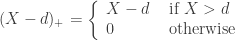
![\begin{array}{rll} E[(X-d)_+] &=& \displaystyle \int_{d}^{\infty}{(x-d)f(x)dx} \\ \\ &=& \displaystyle \int_{d}^{\infty}{S(x)dx} \end{array}](https://s0.wp.com/latex.php?latex=%5Cbegin%7Barray%7D%7Brll%7D+E%5B%28X-d%29_%2B%5D+%26%3D%26+%5Cdisplaystyle+%5Cint_%7Bd%7D%5E%7B%5Cinfty%7D%7B%28x-d%29f%28x%29dx%7D+%5C%5C+%5C%5C+%26%3D%26+%5Cdisplaystyle+%5Cint_%7Bd%7D%5E%7B%5Cinfty%7D%7BS%28x%29dx%7D+%5Cend%7Barray%7D&bg=ffffff&fg=333333&s=0&c=20201002)
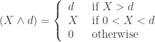
![\begin{array}{rll} E[(X\wedge d)] &=& \displaystyle \int_{0}^{d}{xf(x)dx +dS(x)} \\ \\ &=& \displaystyle \int_{0}^{d}{S(x)dx} \end{array}](https://s0.wp.com/latex.php?latex=%5Cbegin%7Barray%7D%7Brll%7D+E%5B%28X%5Cwedge+d%29%5D+%26%3D%26+%5Cdisplaystyle+%5Cint_%7B0%7D%5E%7Bd%7D%7Bxf%28x%29dx+%2BdS%28x%29%7D+%5C%5C+%5C%5C+%26%3D%26+%5Cdisplaystyle+%5Cint_%7B0%7D%5E%7Bd%7D%7BS%28x%29dx%7D+%5Cend%7Barray%7D&bg=ffffff&fg=333333&s=0&c=20201002)
 .
.![E[X-d|X>d] = \displaystyle \frac{E[(X-d)_+]}{P(X>d)}](https://s0.wp.com/latex.php?latex=E%5BX-d%7CX%3Ed%5D+%3D+%5Cdisplaystyle+%5Cfrac%7BE%5B%28X-d%29_%2B%5D%7D%7BP%28X%3Ed%29%7D&bg=ffffff&fg=333333&s=0&c=20201002)
 and is called
  is called mean residual life in life insurance. Weishaus simplifies the notation by using the P&C notation without the random variable subscript. I’ll use the same.


![\begin{array}{rll} E[X] &=& E[X\wedge d] + E[(X-d)_+] \\ &=& E[X\wedge d] + e(d)[1-F(d)] \end{array}](https://s0.wp.com/latex.php?latex=%5Cbegin%7Barray%7D%7Brll%7D+E%5BX%5D+%26%3D%26+E%5BX%5Cwedge+d%5D+%2B+E%5B%28X-d%29_%2B%5D+%5C%5C+%26%3D%26+E%5BX%5Cwedge+d%5D+%2B+e%28d%29%5B1-F%28d%29%5D+%5Cend%7Barray%7D&bg=ffffff&fg=333333&s=0&c=20201002)
 is said to be shifted by
  is called mean excess loss or mean residual life.
 can be called limited expected value, payment per loss with claims limit, and amount not paid due to deductible.
  and
and  . Any random variables that can only have 2 values is a scaled and translated version of the standard bernoulli distribution.
![E[X] = q](https://s0.wp.com/latex.php?latex=E%5BX%5D+%3D+q&bg=ffffff&fg=333333&s=0&c=20201002) and
and  . If
. If  and
and  with probabilities
  respectively, then
![\begin{array}{rl} Y &= (a-b)X +b \\ E[Y] &= (a-b)E[X] +b \\ Var(Y) &= (a-b)^2Var(X) \\ &= (a-b)^2q(1-q) \end{array}](https://s0.wp.com/latex.php?latex=%5Cbegin%7Barray%7D%7Brl%7D+Y+%26%3D+%28a-b%29X+%2Bb+%5C%5C+E%5BY%5D+%26%3D+%28a-b%29E%5BX%5D+%2Bb+%5C%5C+Var%28Y%29+%26%3D+%28a-b%29%5E2Var%28X%29+%5C%5C+%26%3D+%28a-b%29%5E2q%281-q%29+%5Cend%7Barray%7D&bg=ffffff&fg=333333&s=0&c=20201002)
 and 50%
  ,
,  . This is not the same as
 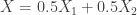 . The latter expression is a sum of random variables NOT a mixture!
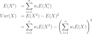
![E[aX+b] = aE[X]+b](https://s0.wp.com/latex.php?latex=E%5BaX%2Bb%5D+%3D+aE%5BX%5D%2Bb&bg=ffffff&fg=333333&s=0&c=20201002)
![E[aX+bY] = aE[X] +bE[Y]](https://s0.wp.com/latex.php?latex=E%5BaX%2BbY%5D+%3D+aE%5BX%5D+%2BbE%5BY%5D&bg=ffffff&fg=333333&s=0&c=20201002)

 are
are  for
for  and
and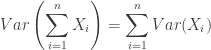
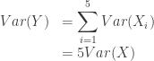 .
.  . In other words,
  is a random variable that takes a value of 5 times the price of AAPL at the close of any given day. Then
 is a random variable over
